Hi.
I'm MJay, from Intel.
In this video, I'm going to introduce the DPDK framework,
a new feature of DPDK that abstracts lower-level features
and helps you seamlessly take advantage of DPDK innovations
faster in your development.
The benefit you get is the portability
of your development across multiple devices
and accelerators, architectures, and generations.
In today's cloud environment, you
might not know what devices are present on a platform.
So this is a critical feature.
DPDK started simple, with Ethernet devices.
Today, with a flex of innovation,
DPDK has expanded to support additional devices
like crypto, compression, SoC, FPGA,
and additional accelerators.
Right now, developers often face challenges
when porting their software to this continuously evolving
scenario.
And that can be really limiting.
Let's give an example.
Let's say a developer wants to deliver a QoS
application on top of DPDK.
Let's assume they do not follow the framework,
and they chose to support only one particular device
in that product.
Once they are done developing the product,
and they start shipping the products to the client,
they learn that the clients are requesting
to use different devices other than the one
the developer chose.
This is not good for the developer.
If their client insist that they want to use a different device,
now the developer has to start porting all over again.
If the developer would have used a DPDK framework,
they would have had a much easier time.
DPDK supports multiple devices from multiple vendors,
and each device has its own unique interface
with this QoS functionality.
That's the problem the DPDK framework solves.
The DPDK framework addresses the community's need
for an abstraction framework.
This abstraction improves agility and portability
for the NFV community.
The main advantage of DPDK is performance.
DPDK framework provides accelerated performance
while abstracting users away from the implementation
details.
In summary, if you write your application
to the DPDK framework, your portability is long-lived.
There's no longer a need to go under the hood
to address specific devices.
Thanks for watching.
Don't forget to access the links provided, to learn more
about the DPDK framework and how it can further benefit you.
For more infomation >> DPDK Framework | Intel Software - Duration: 2:31.-------------------------------------------
God's Word changes everything. || Logos Bible Software - Duration: 1:14.
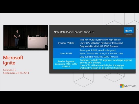
-------------------------------------------
DRÄXLMAIER Group: Software-Entwicklerin Isabelle Roger - Duration: 1:47.
The most exciting thing for me is working on something
and not knowing what you will get in the end.
My name is Isabelle.
I am a software developer at DRÄXLMAIER.
I was born in Paris, but I grew up in England.
I studied in Paris
and after graduating, I came to Germany.
At first to improve my German,
but then I fell in love with the work atmosphere here
so much that I decided to stay.
The challenge
Together with Porsche,
the DRÄXLMAIER Group is developing
the first-ever 800 volt battery
for an electric vehicle
that is going into series production.
That is a completely new technological field
for both companies.
The task
I work on a diagnosis software
It helps determine, for example,
the charging level of the battery.
That's pretty complex,
because it depends on different variables
like temperature or the obsolescence of the cells.
Teamwork
I like working on various concepts in a team.
Everybody approaches a problem differently
and this often helps to solve it.
The fascination
I want to learn new things and
continue to develop myself professionally.
The company continues to put
new mobility technologies on the road,
and this is what I like about DRÄXLMAIER.
-------------------------------------------
Dot Plot by MAQ Software - Power BI Visual Introduction - Duration: 5:00.
Hello and welcome my name is Manuel Quintana with Pragmatic Works, and in
collaboration with MAQ Software, we're bringing you an exciting custom visual
today known as the Dot Plot. This is really going to allow us to isolate and
look at gaps, clustering, and outliers within data by individually plotting
data points on a pretty simple scale, but we have a lot of different varieties and
ways that we can configure and customize this custom visual. Why don't you join
me now in Power BI, so we can take a look at the Dot Plot.
We can see here the Dot Plot by MAQ Software, and there's gonna be multiple
ways that we can show this in regards to orientation. You'll notice here I'm
showing a horizontal orientation, and then just below, we have the exact same
data. This is going to be in our vertical presentation. Let's take a look
and really focus on what's going on within this data, so you can see how nice and
clean and easy this is a way that we can look and find, as we mentioned, outliers,
trends, clustering within our individual data points. Here we can see that we're
talking about various different states and if they're profitable or not. If we
look on the right-hand side, we can see we have various and many, many different
options that we can map our fields to. Right now, we're looking at the axis.
We have our state and then we are looking at the region. We can see at
the very bottom central, east, north, south, and west, of course, and when we hover
over our tooltip gives us tons of information. Here we see our axis—here
the state—but also you'll notice that there's a second. In this case, I've left
axis category 1 available. This is fantastic because we can illustrate how
we can very nicely and easily handle hierarchies here. So now not only are we
looking at this breakdown for state revenue by quarter—and now we're doing
it by region—but now we're doing it by quarter as well. You can see, as you
would expect, the traditional methodology for hierarchy can be leveraged here. I
could kind of keep drilling down these various different categories of year,
quarter, month, and day. Not only that, we have a ton of different configuration
options at our disposal here. Some are gonna be specific whether we're using
the vertical or the horizontal orientation. Let's look at the horizontal
one for right now. When we scroll over, the first option is do we want to keep
it horizontal or do we want to go vertical with it. We also have the
capability of choosing the sorting. This is going to be for the fields that we
put in the axis category one as well as axis category two. We can choose
ascending or descending. Of course, if we continue down the list, you'll find some
very straightforward options. As you would expect, here under access category,
we can go ahead and you notice central, east, north, south, west that was on the
bottom. We've decided that because we've split them, but if we untoggle this, we now
have them together both at the bottom. So this in the
horizontal orientation is going to move it from the top and the
bottom. Within the vertical orientation, it'll move it from left to right.
That's how this is going to work. Of course, all the standard formatting
options as far as coloring, sizing, and font family are going to be available to
us. We also have some interesting items in regards to the jitter effect. We know
about clustering, but in this regard, if we go through and we turn this on, it'll
give just a little bit of an offset to the points that are in that same
location. We can more easily identify these various different groups and
clustering. Notice it is very easy so that you can indicate what is being
highlighted currently. You can set this up so that within the bubbles you have a
selection made for when these items are hovered over. In my case, as I hover over
a specific bubble, it circles it in red, making it only far more easily identifiable.
Something of note that should be indicated here as well is there are some
additional options depending on what we leverage inside of the actual legend
itself. In this regard, we're using "profitable," which is a categorical piece
of data here between nonprofitable and profitable, but if we were to remove this
and bring down a metric like gross margin, you'll notice that we actually
get now this sense of opacity. We can choose the transparency levels here, and
by setting this up and using a metric within the legend, we can go over to the
display area. You'll notice now we have this option for gradient colors—
choosing what is going to be at the low end and what should be at the high end—
and it gives us a gradient scale of colors in between. Of course, tons of
different options. You can see that we can have these various types of
orientation, and it works well with these—you know—small-medium data sets. We
can project and look at these nice scales. What are outliers? How do things
look categorically? We can break down this data very nicely and very easily.
Thanks for watching our video. If you have any questions about this visual or
need a similar business solution, feel free to contact MAQ Software at
sales@maqsoftware.com. As well, for any of your Power BI training needs, be sure to
reach out to us at Pragmatic Works by emailing training@pragmaticworks.com.
-------------------------------------------
Modernize your datacenter with Software-Defined Networking (SDN) in Windows Server - BRK3215 - Duration: 1:12:41.
-------------------------------------------
Forecast using Neural Network by MAQ Software - Power BI Visual Introduction - Duration: 6:24.
Hello and welcome my name is Manuel Quintana with Pragmatic Works, and in
collaboration with MAQ Software, we're bringing you today's video to look at
their custom visual known as Forecast using Neural Network. Now, this is a
fantastic visual, and it starts reaching into the realms of data science and
predictive analytics—which is fantastic—but it is a more advanced
area of conversation. We are gonna see how easy it is to implement this
custom visual right into your Power BI reports and start creating some
predictive analytic visuals, which is fantastic. Now, it should be noted that as
part of this visual you will need to download and install some prerequisites,
but all of this is done easily for you when you go to the Microsoft Store and
you go to install this specific visual. You'll be prompted with a message
letting you know that you do need to have some items installed, and there is a
very nice conveniently located install button right there, and it will go
through that process. What we're doing is we're installing the necessary R
packages for this visual to work. Once that's set and in place, now you can go
ahead and start using this custom visual and looking at data over time, maybe a
different type of data series, and then as well as seeing the data that you have
and you are presenting, we can now predict and get some results back from
what the neural network algorithm has learned. That is what this is all
about: leveraging the neural network learning algorithm, which is also known
like as a black box algorithm or a deep learning algorithm, and it's really great
at looking at nonlinear data. There are quite a few visuals out in the
marketplace that do predictive analytics—and they're more focused around using
algorithms that are great at handling linear data—but where neural network
shines is deriving patterns where it is nonlinear, which can be rather difficult.
Hopefully you're excited and you're ready to enjoy. Let's head over to Power
BI and see how we can put this custom visual into play.
Here we are looking at the Forecast using Neural Network from MAQ Software.
The nature of our data here is just looking at, if we look at the data view,
just the price of gold over time—so over years. Very straightforward, and that's
what we've input. If we look at the field well here for our custom visual, the
series can either be a time or numeric series and then our value. Now do note
that what we're seeing in this teal-ish color—that is our observed values. The
yellow is was what our predicted values are. So to look through this, lets go
right into the format area, so we can have an understanding of where we can
control this. The plot setting is where we can dictate the background color, the
forecast color, and the observed color, which is very important. Of course, we can
control the x and the y axis, but the other main element here is going to be
the forecast settings. Now, the default is setting this to auto, but if you have a
good understanding and you feel confident, you can actually control the
parameters that drive the neural network. We'll look at this momentarily, but I did
want to display it. Once you have this configured—and it should be noted—it
does take some time. Once you define the fields that are going to populate your
visual, the algorithm—the neural network—needs to run. It's going to be doing
analysis and creating predictions of your data. Don't worry if it's taking
a moment; that is the nature of this type of a visual. We can see that we do have
some really neat capabilities with inside of it where we can actually draw
boxes and zoom in to certain elements. By double clicking anywhere in the box, you
go back to your main view. You can enable some spike lines, so as you're moving
across, you can see how that correlates to the rest of the data—how we can see
this is a rise and there's no other peak that equals this one as far as looking
back in time. Of course, you may notice when we zoom in, in this area just
here that we have this little shaded area. This relates to the confidence
intervals. By default, this is turned off, but by turning this on, you now get a
range. You can choose—or you can see we have some confidence levels we can
choose with—lowering this number: having less confidence is gonna narrow this
range. The higher the number we're giving ourselves a little more breathing
room saying hey we're confident that the values in this time frame will fall
between these little brackets, and as you hover over,
you can see the information. The confidence level here for 2016 is gonna
be that 1373 and some change, while the yellow line is just the raw
predicted line. Really neat, really powerful, but as I mentioned, we could go
even further. If we look at the same visual but in the context of going over
to the format area and choosing to switch the forecast settings from auto
to user-defined, we have a couple of choices here. Now, of course, there's a lot
that goes into data science and learning, but we have some items here where
decay kind of controls the learning rate of the neural network. The maximum
number of iterations is how many times it's gonna run these numbers through the
neural network and coming up with different values and then coming back
with the best distribution. The number of units, in this case, is gonna represent
our series, which were going in years, so this is going to predict out to ten
years from where we ended our observed. Of course, epochs is going to be the kind
of rotations, so we're gonna have two hundred iterations over a single epoch.
Here, we're gonna have eight epochs. Lowering these values, of course, has less
iterations—there's less loading time—but there is this concept of overfitting,
which can occur if you start increasing these numbers. Basically, you're making it
learn the specifics of this data, so when new data is introduced, it may not
interpret that as correctly. Like I said, we're working in the realm of data
science, so there's a lot of information to understand here, but hopefully you can
see very quickly and how easily you can now already start using data science or
predictive model visuals here right within Power BI with the usage of this
Forecast using Neural Networks by MAQ Software. Hopefully you enjoyed, and thanks
for watching our video. If you have any questions about this visual or need a
similar business solution, feel free to contact MAQ Software at sales@maqsoftware.com.
As well, for any of your Power BI training needs, be sure to reach
out to us at Pragmatic Works by emailing training@pragmaticworks.com.
Không có nhận xét nào:
Đăng nhận xét